Introduction
A novel methodology for carbonate reservoir characterization based on the empirical relationships between pore types and reservoir parameters has been developed. The method is integrated into a geological framework and therefore gives sedimentological/diagenetic control on reservoir quality distribution. The new methodology is applied to predict pore types, permeability, effective porosity, porosity cut-off, capillary pressures, saturations, HC contacts, FWL, HC volumes and more. For many of these parameters the expected and P10 to P90 values are predicted, along with the standard deviations. The method can be applied in both production and exploration scenarios and produces detailed input parameters to reservoir modeling. STOOIP/GIIP calculations and sensitivity testing can be carried out in short time based on measured and/or predicted input values at wire-line log resolution and without the need of any vertical up-scaling. The method was accepted by BeicipFran Lab. in a 2012 audit of a producing reservoir, and has been successfully applied to one Russian, four Iranian, four Iraqi and two UAE oil and gas fields. It has also been applied in the application for the 22nd and 23rd Norwegian license rounds and in project evaluation in the Norwegian Sea exploration.
Prediction tools involved in the new methodology have been compiled into a WEB-based program called CARP (CArbonate Reservoir Properties), which is accessible from the emnu item "Prediction Tools".
Pore Types
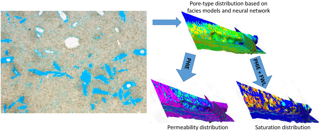
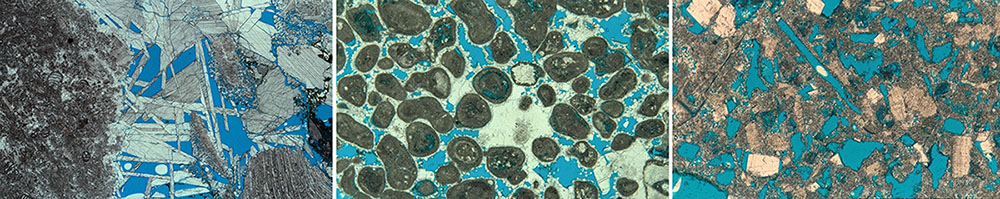
Pore types are normally defined from thin sections and predicted from wire-line logs in non-cored intervals using artificial neural network (ANN). In limited data sets they can also be predicted, with lower accuracy, from porosity-permeability relationships. In exploration pore types are based on regional experience and/or sedimentological/diagenetic models. The applied pore-type classification system is published in: Lønøy, A., 2006. Making sense of carbonate pore systems: AAPG Bulletin, v. 90, no. 9 (September 2006), pp. 1381–1405.
ANN-prediction of pore types has been carried out on several fields and shows that pore types usually are correctly predicted in 70-80% of the samples when 6-8 pore types or pore-type groups are present in the data set. This high prediction accuracy has been verified in test data and blind test wells.
Both a dominant and, if relevant, a subordinate pore type are defined from thin sections and predicted from ANN. Defining up to two important pore-type constituents improves prediction.
The pore types are integrated into sedimentologic models in order to distribute pore types between wells. Porosity histograms for different pore types are used to optimize the integrated pore type and porosity distribution between wells (to avoid that pore types and porosity are distributed independently from each other).
Permeability
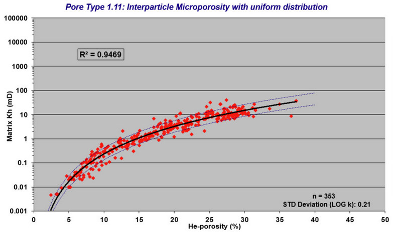
Permeability prediction is based on empirical global relationships between pore types, porosity and permeability. Expected and P10 to P90 permeabilities are predicted and are based on a revision of Lønøy (2006). The permeability prediction tool can handle up to two important pore types (dominant and subordinate).
Plug-measured permeabilities in a given reservoir are always applied to test the validity of the global equations. If needed, the equations are modified to honor the measured data.
Effective Porosity
Total porosity is composed of effective and ineffective porosity (PHItotal = PHIeffective + PHIineffective). Ineffective porosity is believed to have insufficient permeability to contribute to flow.
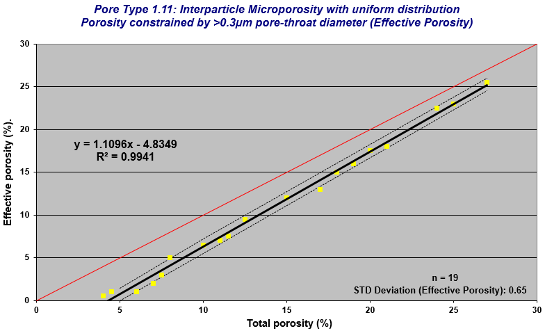
The effective porosity is controlled by pore-throat diameter, where porosity enclosed by pore-throat diameters less than a specific limit is considered ineffective. Essentially, a cut-off on pore-throat diameter is applied. There are several other factors which will have an effect on effective porosity (e.g. viscosity, oil composition, pressures, wetting and turtoisity) but these are not considered here.
Pore-throat diameters and effective porosity are dependent on pore type and porosity, and can be determined from mercury injected capillary pressure (MICP) curves. Based on a large global database, the relation between effective and total porosity for different pore types has been defined. The effective porosity is defined as the total Hg-injected pore volume minus the pore volume constrained by a specific pore-throat diameter. Pore-throat diameter cut-offs of 0.3 and 0.6 µm have been applied.
The effective porosity tool can handle up to two important pore types (dominant and subordinate) and predicts expected and P10 to P90 effective porosity at two different pore-throat cut-offs. Measured MICP data for a given reservoir are applied to test the validity of the global equations. If needed, the equations are modified to honor the measured data.
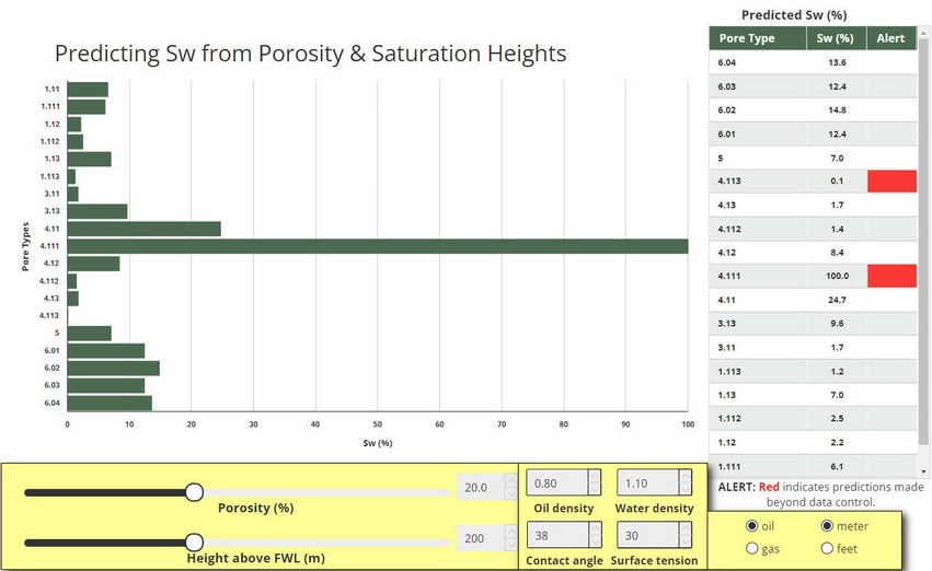
Saturation
Saturation is based on MICP-based saturation heights. Several methods can be applied in averaging the measured capillary pressure curves, e.g. Leverett J-function, Thomeer, and empirical global functions based on pore-type composition (unpublished methodology developed by A. Lønøy – subsequently called the Lonoy method).
The Lonoy method is based on empirical relations between pore types, porosity and MICP curves, and applies a large, global, carbonate data set. Best fit equations for MICP curves and irreducible water saturation (Swirr) have been optimized for porosities up to 30%. The advantage of this method is that permeability is not required as input and that the MICP curve can be predicted from porosity and pore type (both dominant and subordinate pore types can be handled).
Measured MICP data for a given reservoir are applied to test the validity of the global saturation equations. If needed, the equations are modified to honor the measured data. By comparing the measured data to the global equations, the prediction error can be calculated for different parts of the reservoir.
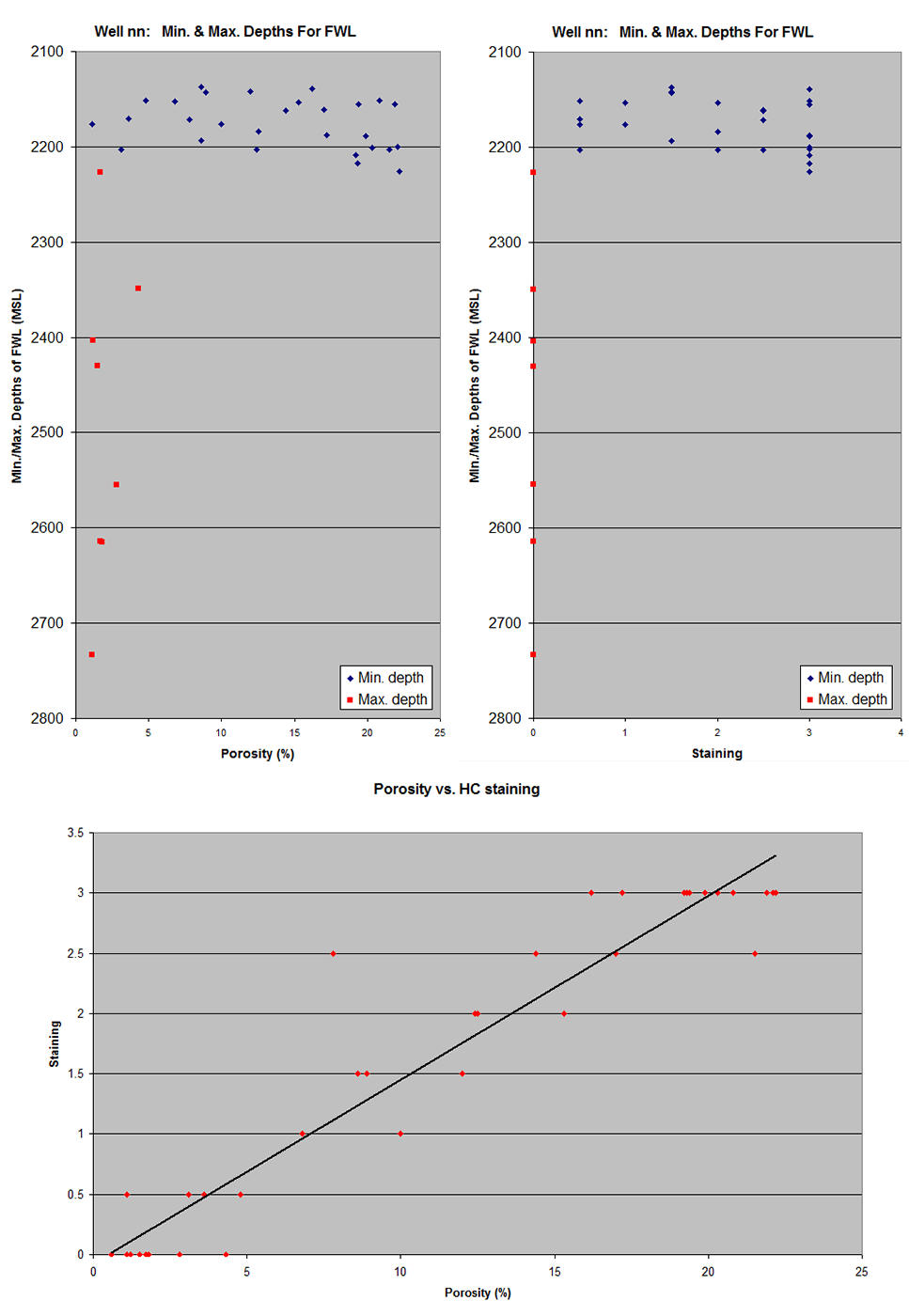
FWL
If pressure gradients are unavailable the free water level (FWL) may to some extent be predicted from MICP curves (either measured or predicted from porosity and pore types) and associated hydrocarbon staining of core material. It is not an exact method, but has proven to be useful in some cases.
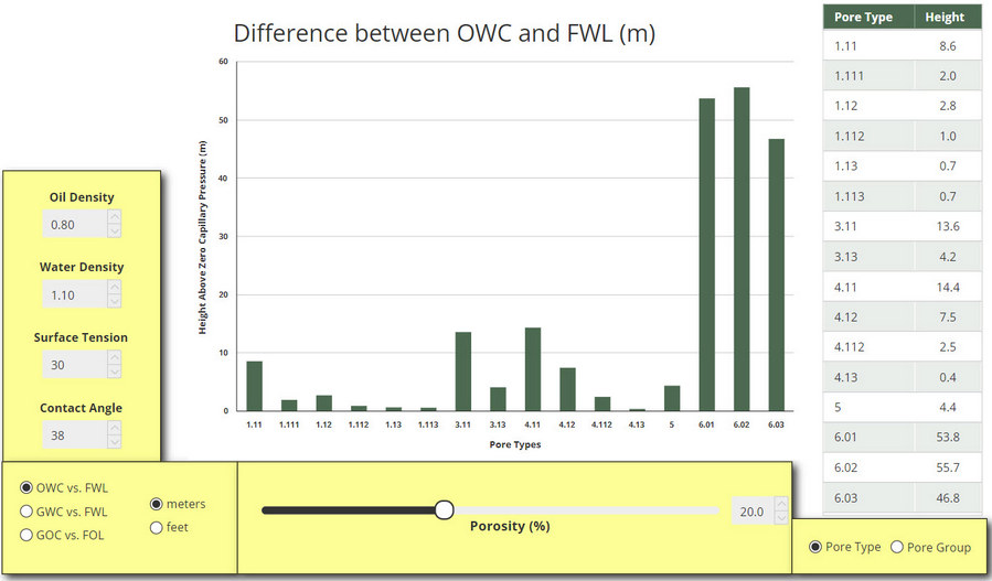
HC Contacts
The location of the HC contacts relative to FWL (free water level) and FOL (free oil level) is strongly controlled by pore types, porosity and wetting. In carbonate reservoirs the OWC (oil-water contact) may be up to several hundreds of meter away from the FWL, depending on the reservoir quality. With detailed knowledge on porosity and pore-type distribution within the reservoir, the location of HC contacts within the reservoir can be predicted. The limitation in prediction is primarily related to uncertainties in wetting.
HC Volumes
Traditional methods for estimating STOOIP and GIIP is based on the use of average input parameters for different reservoir zones, and by the application of a variety of cut-offs in net-to gross evaluations. This methodology creates a significant uncertainty in the volume calculations, especially related to saturation, up-scaling, and to the application of cut-offs.
A new methodology has been developed for estimating matrix-related HC volumes and for predicting the sensitivity of the estimates. The methodology is developed by A. Lønøy and is unpublished. The method does not apply fixed input parameters, but uses measured and/or predicted pore-type related input parameters that vary continuously through the reservoir. Well data are normally preferred as input data, although it is possible to use data from geological models. The methodology is to a large degree based on pore-type control of reservoir parameters.
The basic elements of traditional volume estimation are applied in the new methodology (STOOIP will be used as an example):
- STOOIP = BRV * Φ * So * 1/Bo (Equation 1)
where BRV = Bulk Rock Volume, Φ = Porosity, So = Oil Saturation, and Bo = Formation Volume Factor.
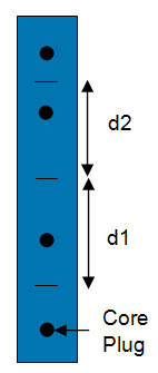
In the new method the reservoir is subdivided into several thin depth zones, where the number of zones equals the number of samples available. A sample may be a core plug, core chip or wire-line log reading, and the thickness of each zone is defined by the mid-point between the samples (e.g. d1 and d2 in the figure) or by stratigraphic breaks. Different porosities, oil saturations and formation volume factors may be applied to each zone.
Equation 1 can be written as:
- STOOIP = BRV * SF (Equation 2)
- SF = Φ * So * 1/Bo (Equation 3)
where SF = STOOIP factor
A partial STOOIP factor (SFp) is calculated for each interval, using the reservoir parameters for the interval (interval d1 given as an example in equation 4):
- SFp (1) = * So * d1/(d1 + d2 + …. + dn) / Bo (Equation 4)
where d1 is the thickness of zone 1, and dn is the thickness of the last zone (n = number of samples).
The partial STOOIP factors add up into a total reservoir STOOIP factor:
- SF = SFp (1) + SFp (2) + .... + SFp (n) (Equation 5)
This total STOOIP factor is applied in equation 2 to calculate the STOOIP of the reservoir.
As can be seen from the equations above, the porosity, oil saturation and formation volume factor may be specified for each thin reservoir interval.
Oil Saturation
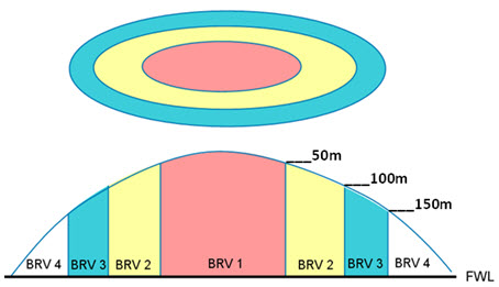
The oil saturation will vary according to structural position. For a given stratigraphic unit the oil saturation will be highest at the structural apex (assuming constant reservoir properties across the field), and will gradually decrease down flank. The saturation predicted within a well will thus only be valid for the well location. To ensure correct prediction of saturation across the field, the saturation is predicted at different structural positions, defined by user-definable depth contours of top reservoir (usually 50 or 100m incremental depth contours, starting from the structural apex).
The bulk rock volume (BRV) is split into vertical segments, which are constrained by depth contours, cap rock and FWL (see birds-eye view and cross-section in figure). For each vertical segment the corresponding distribution of oil saturation is applied.
HC Volume Estimation & Sensistivity Testing
The final HC volume estimation and sensitivity testing is carried out within an automated, macro-based Excel spreadsheet. The partial STOOIP/GIIP for each vertical segment is calculated using the saturation distribution at the intermediate depth contour of each segment, and the total STOOIP/GIIP is the sum of the partial STOOIPs/GIIPs.
Any type of cut-off can be implemented in the model and the advantage, as compared to traditional methods, is that the use of pore types and their associated porosity-permeability relationships (Lønøy, 2006) makes it possible to apply a direct permeability cut-off. Permeabilities are given to each sample in the model, either as a measured value or as an estimated value based on Lønøy (2006). Traditional methodology for estimating HC volumes usually applies a porosity cut-off based on porosity-permeability cross-plots for samples covering a wide range of pore types. This is inaccurate, as different pore types have different porosity-permeability relationships.
Pore-type distributions and any other inputs can easily be changed in the model, and recalculated STOOIP/GIIP calculations can be made in seconds to few minutes. This allows for easy and rapid sensitivity of the input parameters. The model can handle oil reservoirs, gas reservoirs and oil reservoirs with a gas cap.
Limitations of the Model
One of the limitations of the model is that the input data are applied to the entire field, regardless of lateral variations. The calculated HC volumes are only correct if the applied input data are representative for the entire field. This problem can be minimized by dividing the field into regional segments and apply one model to each segment. This can be accomplished by applying well data from several wells, or by using estimated input data (pseudo wells) derived from geological models. The total HC volume will then be the average of the individual well-based HC volumes, or a proportional HC volume contribution based on each well’s relative contribution.
Reservoir Models
The final reservoir model is based on the spatial distribution of pore types and porosity across the field. The distribution is controlled by well data and sedimentological/diagenetic models. Once the porosity and pore types have been distributed, all other parameters are equation based (e.g. permeability, effective porosity and saturation).